Watershed Network Analysis: Part 1

Natural Resources, Nutrient Loading and NetworkX

1. Introduction: Natural Resources | Data Science

In making the exciting (and sometimes daunting) journey through an interdisciplinary PhD program in Natural Resources with a dual focus in Ecological Economics and Complex Systems, I have a tremendous appreciation for the opportunity to engage with the Earth Science Information Partners community. Being an ESIP Student Fellow has helped me navigate the complicated waters between earth science and data science, first in the Agriculture and Climate Cluster and now in the Earth Science Data Analytics Cluster.

In this two-part Watershed Network Analysis blog series, I highlight connections between earth science, natural resource management, and data science – and how I've come to find myself here at the crossroads. Perhaps more importantly, I hope to demonstrate why it may be useful to explore the application of network analysis methods predominantly used in “big data” data science, to natural resource management.

Which brings us to: pretty figures Exciting Data Science Tools & Natural Resource Applications

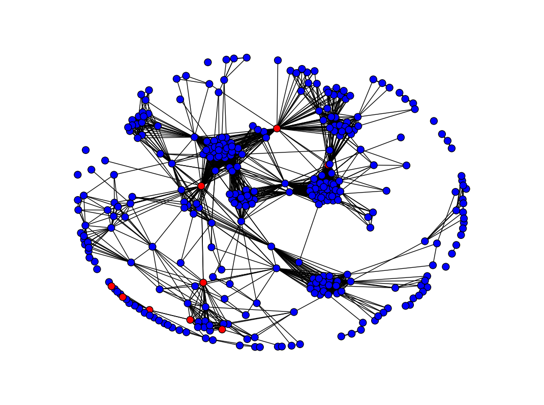
Figure 1 LaPlatte Watershed Network: a peek to pique interest

2. Agriculture and Water:

In a previous blog post I discussed  my research on agriculture and climate through use of in-field and remote sensing techniques (like Drones!) to help monitor greenhouse gas emissions. However, agriculture impacts many environmental systems:

Water. Another major aspect of my research involves managing the effects of agricultural inputs (fertilizer and manure) on water quality (runoff into rivers and lakes). I monitor manure application methods to determine the best field management strategies for reducing agricultural runoff.

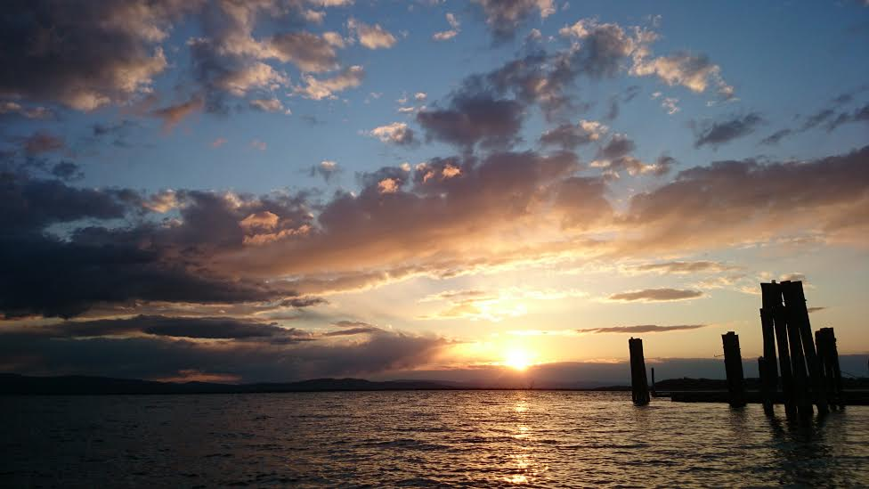
Figure 2 Photograph taken while kayaking on Lake Champlain. Come visit anytime. 

Surrounded by three agricultural regions (Vermont and New York as well as Canada’s province of Quebec) Lake Champlain experiences many negative effects of agricultural runoff. Nutrients, such as phosphorus and nitrogen are transported from the land, into streams and rivers, and ultimately to the lake. In excess, these nutrients cause eutrophic conditions and algal blooms, which can disrupt recreation, cause fish die-offs, decrease biodiversity, and release toxins that can cause illness and animal mortality.

And it’s not just Lake Champlain. Surveys have shown eutrophic conditions in 48% of lakes in North America. And it’s not just North America. Surveys have shown eutrophic conditions in 54% of lakes in Asia, 53% of lakes in Europe, 41% of lakes in South America, and 28% of lakes in Africa. And it’s not limited to lakes either – the World Resources Institute has identified 375 hypoxic coastal zones in the world due to eutrophication.

3. Land and Nutrient Export:

Land use and land cover are well-known determinants of nutrient export and subsequent loading in rivers and lakes, and certain land types are known to export more nutrients than others on average. For example, The Lake Champlain Basin Program uses this equation:

TLD = ECK * A

Where:

TLD = total annual load for a cell (kg)

ECK = export coefficient for land use K

A = area of the cell (constant of 0.09 ha)

Average export coefficients are assigned to each Land Use / Land Cover map on a cell-by-cell basis and then used to produce an export value for each cell in kg/yr. Cropland and Hay/Pastureland are two of the land cover types that have the highest nutrient export coefficients. Forests export much less and can even serve to mitigate runoff when planted in areas along rivers – known as riparian buffer zones.

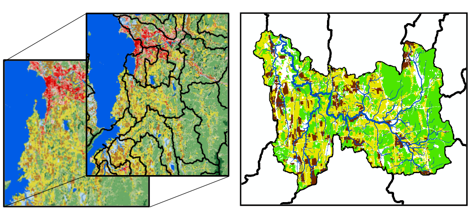
Therefore, to begin visualizing where and how nutrients are transported across the landscape, it is useful to start with the most recent National Land Cover Database (NLCD 2011).

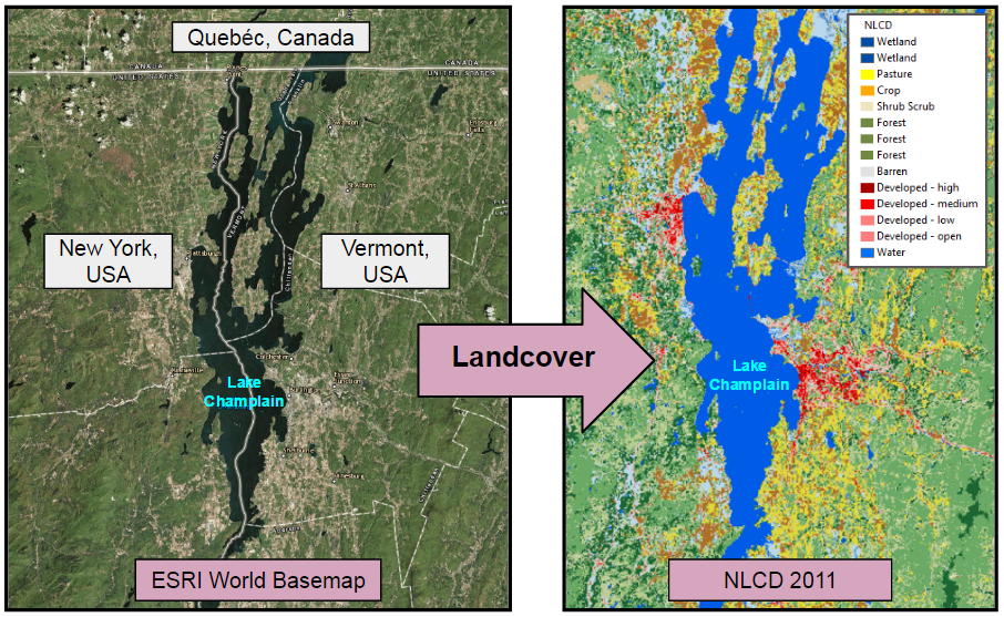
Figure 3 Lake Champlain Basin Landcover

However, predictive equations and export coefficients vary greatly and depend on many stochastic factors, including precipitation and actual land management practices (Troy, 2007). Rivers and streams are the main transport network of nutrients into the lake, so understanding how land interacts spatially with the river system in a watershed is a necessary step in assessing nutrient export on a landscape scale.

While this sort of spatial analysis is often done in ArcGIS, or using domain-specific models such as SWAT, RHESSys or InVEST, I wanted to explore the use of more abstracted network analysis techniques typically used in the realm of Data Science.

4. Network & Graph Theory: Background

Graph Theory dates back to Leonhard Euler in 1736, with a really concrete foundation story:

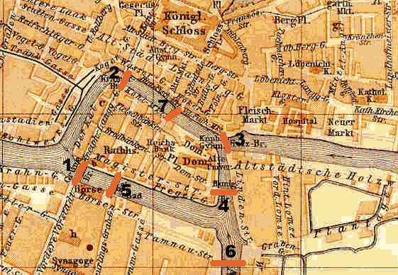
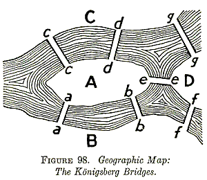
Figures 4 & 5 Baedeker, Atlas of Northern Germany, 1890 & Kraitchik, 1942

”The Königsberg bridge problem asks if the seven bridges of the city of Königsberg over the river Preger can all be traversed in a single trip without doubling back, with the additional requirement that the trip ends in the same place it began. This is equivalent to asking if the multigraph on four nodes and seven edges has an Eulerian cycle. This problem was answered in the negative by Euler (1736), and represented the beginning of graph theory.” (Weisstein, Eric W. “Königsberg Bridge Problem.” From MathWorld–A Wolfram Web Resource)

Perhaps not the most well-worded story, but there you go.

Graph-theoretic abstraction and subsequent analysis has been used to study networks of all kinds. With nodes representing individual members of the network, and links between nodes representing connections between those members, once the network is established, algorithms can then be used to explore and ascertain the structure of the network. For example one can determine:

• on average how many connections nodes have with each other

• the presence and structure of communities within the network

• nodes that are “hubs” for connecting different clusters of other nodes

There have been many applications of these techniques to explore social networks. One great (and ESIP-relevant) example is a recent AGU blog post that shows connections between ESSI coauthors on AGU abstracts.

However, I am particularly interested in exploring these techniques to answer questions relating to environmental networks. Which brings us back to:

5. Watershed Network Analysis: The Setup in Two Steps

Step One: The Study Site

The LaPlatte Watershed in Vermont.

Three NLCD land cover types were used in this analysis: Forest, Crop, and Hay/Pasture. The LaPlatte Watershed contains 281,943m of rivers, draining a total area of 145 km2. This river network is comprised of 727 river reaches. River Reaches? The term “reach” is used to characterize rivers into geomorphologically distinct segments. Reaches are identified by unique “reach codes”. This helps us “reach” for connections between land patches and river segments, and will be particularly important when analyzing the watershed network.

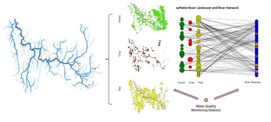
Step Two: Spatial to Graph

LaPlatte Watershed: from spatial data to a bipartite network using ArcGIS and Python: NetworkX.

Each NLCD land cover patch is represented as a node in the bipartite network, where land cover nodes are connected to river nodes if the land patch is spatially connected to the river reach. Node size is based on a threshold of 40 hectares with larger patches corresponding to larger nodes.

In-stream water chemistry and nutrient data were then connected to the river reaches that were monitored for water quality. This allows for the linking of nutrient concentrations in the river to land cover information to help identify:

• potential river and land patch “hotspots” to help target mitigation efforts (e.g. planting riparian buffer zones)

• the role of adjacent and upstream land patches on nutrient levels measured in particular segments of the river network to improve water quality predictions

• river and land patch targets for multi-purpose conservation (e.g. connecting forest patches along waterways to help improve water quality while also increasing habitat connectivity)

To be explored in:

Watershed Network Analysis: Part 2

Analyzing the Network & Assessments of Water Quality and Conservation Priority Areas

Stay tuned.

with thanks to Dr. James Bagrow and Keri Watson

—

Did you make it this far? Want to discuss any of this? Collaborate on a project? See my code?

twitter: @barbieriiv

email: lindsay.barbieri@uvm.edu

or better yet, register for this awesome conference: ESIP Summer Meeting and let’s talk in July!

I would love to talk more about: Earth Science: Environment, Natural Resources, Agriculture & Climate. Data Analysis: Techniques — (Networks, Statistical Learning Methods and Data Imputation Techniques) Tools — (Python & R – Having weird issues with bipartite graphs in NetworkX? Ever used R package CausalImpact?) Spatial — ArcGIS, eCognition, Dinamica, or are you using Python or R for image processing? Data Management: Help