Deadline Friday! Apply for the ESIP Raskin Scholarship by March 13. Learn more and apply.
pysheds: a fast, open-source digital elevation model processing library
Hey ESIP!
I wanted to share a pet project of mine that could be useful for those of you who work with GIS data (and especially for those of you who work with water data of any kind).
Pysheds is an open-source library designed to help with processing of digital elevation models (DEMs), particularly for hydrologic analysis. Pysheds performs many of the basic hydrologic functions offered by commercial software such as ArcGIS, including catchment delineation and accumulation computation.
I designed pysheds with speed in mind. It can delineate a flow direction grid of ~10 million cells in less than 5 seconds. Flow accumulation for a grid of 36 million cells can be computed in about 15 seconds. These methods can be readily automated and incorporated into web services: for instance, a web mapping service like leaflet.js could use pysheds to generate contributing areas for locations of interest on-the-fly.
The library is available at my github here: https://github.com/mdbartos/pysheds
A full feature list is given below:
- Hydrologic Functions:
flowdir: DEM to flow direction.catchment: Delineate catchment from flow direction.accumulation: Flow direction to flow accumulation.flow_distance: Compute flow distance to outlet.resolve_flats: Resolve flats in a DEM using the modified method of Garbrecht and Martz (1997).fraction: Compute fractional contributing area between differently-sized grids.extract_river_network: Extract river network at a given accumulation threshold.cell_area: Compute (projected) area of cells.cell_distances: Compute (projected) channel length within cells.cell_dh: Compute the elevation change between cells.cell_slopes: Compute the slopes of cells.
- Utilities:
view: Returns a view of a dataset at a given bounding box and resolution.clip_to: Clip the current view to the extent of nonzero values in a given dataset.resize: Resize a dataset to a new resolution.rasterize: Convert a vector dataset to a raster dataset.polygonize: Convert a raster dataset to a vector dataset.check_cycles: Check for cycles in a flow direction grid.set_nodata: Set nodata value for a dataset.
- I/O:
read_ascii: Reads ascii gridded data.read_raster: Reads raster gridded data.to_ascii: Write grids to ascii files.
An overview with examples is given here:
Import modules
import numpy as np
import pandas as pd
from pysheds.grid import Grid
import geopandas as gpd
from shapely import geometry, ops
import matplotlib.pyplot as plt
import matplotlib.colors as colors
import seaborn as sns

import warnings
warnings.filterwarnings('ignore')
sns.set_palette('husl')

%matplotlib inline
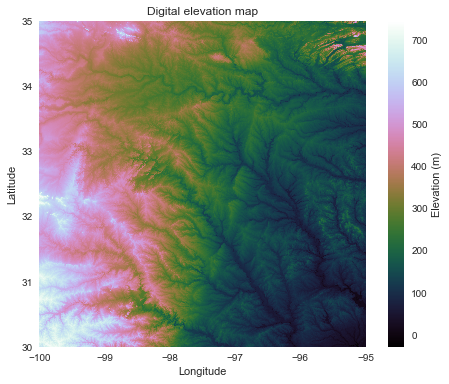
Instantiate a grid from a DEM raster
Data from USGS hydrosheds project: https://hydrosheds.cr.usgs.gov/datadownload.php
# Instatiate a grid from a raster
grid = Grid.from_raster('../data/n30w100_con', data_name='dem')
# Plot the raw DEM data
fig, ax = plt.subplots(figsize=(8,6))
plt.imshow(grid.dem, extent=grid.extent, cmap='cubehelix', zorder=1)
plt.colorbar(label='Elevation (m)')
plt.title('Digital elevation map')
plt.xlabel('Longitude')
plt.ylabel('Latitude')
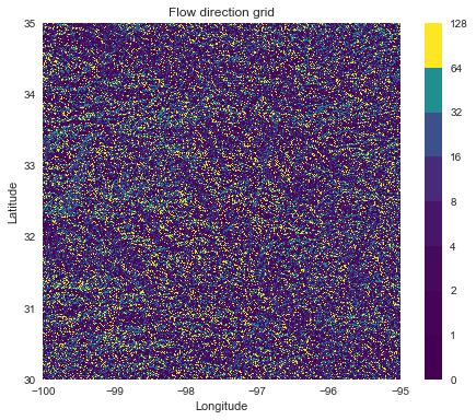
Read a flow direction grid from a raster
Data from USGS hydrosheds project: https://hydrosheds.cr.usgs.gov/datadownload.php
# Read a raster into the current grid
grid.read_raster('../data/n30w100_dir', data_name='dir')
Examine grid
# The flow direction raster is contained in a named attribute (in memory)
grid.dir
Raster([[ 64,  64,  64, ...,   1,   2, 128],
        [ 32,  64,  64, ...,   1,   1, 128],
        [ 32,  32,  32, ...,   1, 128,  64],
        ...,
        [128,  64,  64, ...,  16,   8,   4],
        [128,  64,  64, ...,   4,  16,   4],
        [  8,  64,  64, ...,   8,   4,   4]], dtype=uint8)
# There are approximately 36 million grid cells
grid.dir.size
36000000
Specify flow direction values
#N    NE    E    SE    S    SW    W    NW
dirmap = (64,  128,  1,   2,    4,   8,    16,  32)
Examine grid
# Access the flow direction grid
fdir = grid.dir

# Plot the flow direction grid
fig = plt.figure(figsize=(8,6))
plt.imshow(fdir, extent=grid.extent, cmap='viridis', zorder=1)
boundaries = ([0] + sorted(list(dirmap)))
plt.colorbar(boundaries= boundaries,
             values=sorted(dirmap))
plt.title('Flow direction grid')
plt.xlabel('Longitude')
plt.ylabel('Latitude')
Delineate catchment
# Specify pour point
x, y = -97.294167, 32.73750

# Delineate the catchment
grid.catchment(data='dir', x=x, y=y, dirmap=dirmap, out_name='catch',
               recursionlimit=15000, xytype='label', nodata_out=0)
# Clip the bounding box to the catchment
grid.clip_to('catch')
# Get a view of the catchment corresponding to the current bounding box
catch = grid.view('catch', nodata=np.nan)
# Plot the catchment
fig, ax = plt.subplots(figsize=(8,6))
im = ax.imshow(catch, extent=grid.extent, zorder=1, cmap='viridis')
plt.colorbar(im, ax=ax, boundaries=boundaries, values=sorted(dirmap),
             label='Flow Direction')
plt.title('Delineated Catchment')
plt.xlabel('Longitude')
plt.ylabel('Latitude')

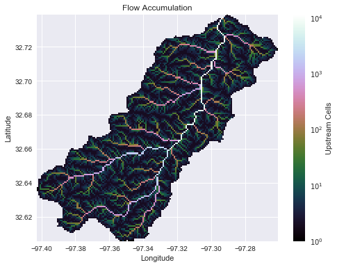
Get flow accumulation
# Compute flow accumulation at each cell
grid.accumulation(data='catch', dirmap=dirmap, out_name='acc')
# Get a view and add 1 (to help with log-scaled colors)
acc = grid.view('acc', nodata=np.nan) + 1

# Plot the result
fig, ax = plt.subplots(figsize=(8,6))
im = ax.imshow(acc, extent=grid.extent, zorder=1,
               cmap='cubehelix',
               norm=colors.LogNorm(1, grid.acc.max()))
plt.colorbar(im, ax=ax, label='Upstream Cells')
plt.title('Flow Accumulation')
plt.xlabel('Longitude')
plt.ylabel('Latitude')
Extract river network
# Extract branches for a given catchment
branches = grid.extract_river_network(fdir='catch', acc='acc',
                                      threshold=50, dirmap=dirmap)
# Plot the result
fig, ax = plt.subplots(figsize=(6.5,6.5))
plt.title('River network (>50 accumulation)')
plt.xlabel('Longitude')
plt.ylabel('Latitude')
plt.xlim(grid.bbox[0], grid.bbox[2])
plt.ylim(grid.bbox[1], grid.bbox[3])
ax.set_aspect('equal')
for branch in branches['features']:
    line = np.asarray(branch['geometry']['coordinates'])
    plt.plot(line[:, 0], line[:, 1])

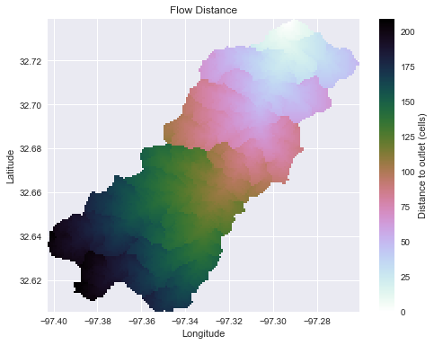
Get distances to upstream cells
# Compute flow distance using graph traversal
grid.flow_distance(data='catch', x=x, y=y, dirmap=dirmap, out_name='dist',
                   xytype='label', nodata_out=np.nan)
# Return a view of the flow distance grid
dist = grid.view('dist', nodata=np.nan)

# Plot the result
fig, ax = plt.subplots(figsize=(8,6))
im = ax.imshow(dist, extent=grid.extent, zorder=1,
               cmap='cubehelix_r')
plt.colorbar(im, ax=ax, label='Distance to outlet (cells)')
plt.title('Flow Distance')
plt.xlabel('Longitude')
plt.ylabel('Latitude')
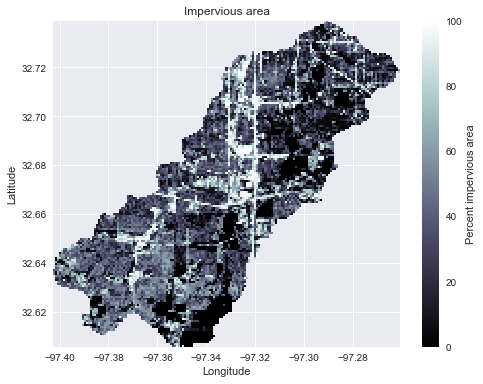
Combine with land cover data
Data available here: https://www.mrlc.gov/nlcd2011.php
# Read land cover raster
grid.read_raster('../data/impervious_area/nlcd_2011_impervious_2011_edition_2014_10_10.img',
                 data_name='terrain', window=grid.bbox, window_crs=grid.crs)
interpolated_terrain = grid.view('terrain', nodata=np.nan)

fig, ax = plt.subplots(figsize=(8,6))
plt.imshow(interpolated_terrain, cmap='bone', zorder=1,
           extent=grid.extent)
plt.colorbar(label='Percent impervious area')
plt.title('Impervious area')
plt.xlabel('Longitude')
plt.ylabel('Latitude')
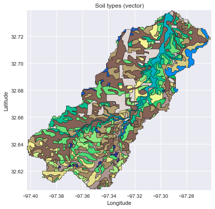
Clip soils shapefile to catchment
Data available here: https://tnris.org/data-download/#!/county/Tarrant
# Read soil dataset
soils = gpd.read_file('../data/nrcs-soils/nrcs-soils-tarrant_439.shp')
soil_id = 'MUKEY'
# Convert catchment raster to vector geometry and find intersection
shapes = grid.polygonize()
catchment_polygon = ops.unary_union([geometry.shape(shape)
                                     for shape, value in shapes])
soils = soils[soils.intersects(catchment_polygon)]
catchment_soils = gpd.GeoDataFrame(soils[soil_id],
                                   geometry=(soils.geometry
                                             .intersection(catchment_polygon)))
# Convert soil types to consecutive integer values
soil_types = np.unique(catchment_soils[soil_id])
soil_types = pd.Series(np.arange(soil_types.size), index=soil_types)
catchment_soils[soil_id] = catchment_soils[soil_id].map(soil_types)
# Plot the result
fig, ax = plt.subplots(figsize=(6.5, 6.5))
catchment_soils.plot(ax=ax, column=soil_id, categorical=True,
                     cmap='terrain', linewidth=0.5, alpha=1)
ax.set_xlim(grid.bbox[0], grid.bbox[2])
ax.set_ylim(grid.bbox[1], grid.bbox[3])
ax.set_title('Soil types (vector)')
plt.xlabel('Longitude')
plt.ylabel('Latitude')
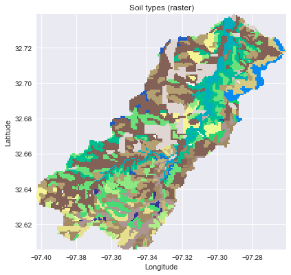
Rasterize soil data in catchment
# Rasterize the soil polygons
soil_polygons = zip(catchment_soils.geometry.values,
                    catchment_soils[soil_id].astype(int).values)
soil_raster = grid.rasterize(soil_polygons, fill=np.nan)
# Plot the result
fig, ax = plt.subplots(figsize=(6.5, 6.5))
plt.imshow(soil_raster, cmap='terrain', extent=grid.extent, zorder=1)
ax.set_xlim(grid.bbox[0], grid.bbox[2])
ax.set_ylim(grid.bbox[1], grid.bbox[3])
ax.set_title('Soil types (raster)')
plt.xlabel('Longitude')
plt.ylabel('Latitude')